Ribbon过滤器原理解析

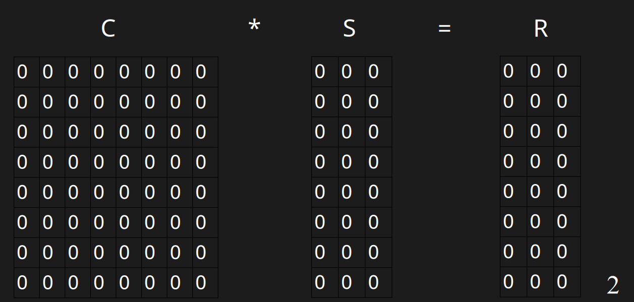
Ribbon过滤器整体看是一个矩阵构建与矩阵乘法，RocksDB中对它的实现是进行了合理的空间、时间上的优化的。 ## 符号 整个过滤器都和矩阵计算CS=R相关，C是\(n\*n\)矩阵，S是\(n\*m\)矩阵，R是\(n\*m\)矩阵。 这里为了方便讨论定义：三个哈希函数s(x),c(x),r(x)，s是start函数，c是coeff函数，r是result函数。其中c的返回值是一个定长二进制整数，比如c(x)返回0010，那么c(x)返回的整数是长度为w=4的二进制整数。 此外为了方便讨论，我们假定n=8, m=3，h(x)为s(x)个0拼接c(x)拼接n-w-s(x)个0。比如： | key | s(x) | c(x) | r(x) | h(x) | | --- | --- | --- | --- | --- | | u | 0 | 1000 | 000 | 1000 0000 | | v | 0 | 1100 | 111 | 1100 0000 | | w | 0 | 1010 | 100 | 1010 0000 | | x | 3 | 1000 | 101 | 000 1000 0 | | y | 0 | 1001 | 111 | 1001 0000 | ## 构建过程 构建过程本质上是解一个CS=R的矩阵乘法。C和R是由插入的键构建的，S是C和R解出来的。这里定义的矩阵乘法是： \[c\_{ij} = \bigoplus\_{k=1}^{n} (a\_{ik} \land b\_{kj}) \] 与原本的矩阵乘法非常相似，就是乘法变成逻辑与，加法改成逻辑xor罢了。 \[c\_{ij} = \sum\_{k=1}^{n} a\_{ik} b\_{kj} \] ### 初始化 初始化，默认所有值为0  ### 插入过程 ```python def leading_zeros_count(self, vec: np.matrix): for i in range(vec.shape[1]): if vec[0, i] != 0: return i return vec.shape[1] def banding_add(self, h, resultrow): print(h, resultrow) while True: start = self.leading_zeros_count(h) if np.all(h[0] == 0): if np.all(resultrow[0] == 0): break else: raise ValueError("cannot insert this row") elif np.all(self.coeff[start] == 0): # 如果start这一行全是0，就把这一行赋值为coeffrow self.coeff[start] = h self.result[start] = resultrow break else: h = self.row_xor(h, self.coeff[start]) resultrow = self.row_xor(resultrow, self.result[start]) print(self.coeff) print(self.result) ``` #### 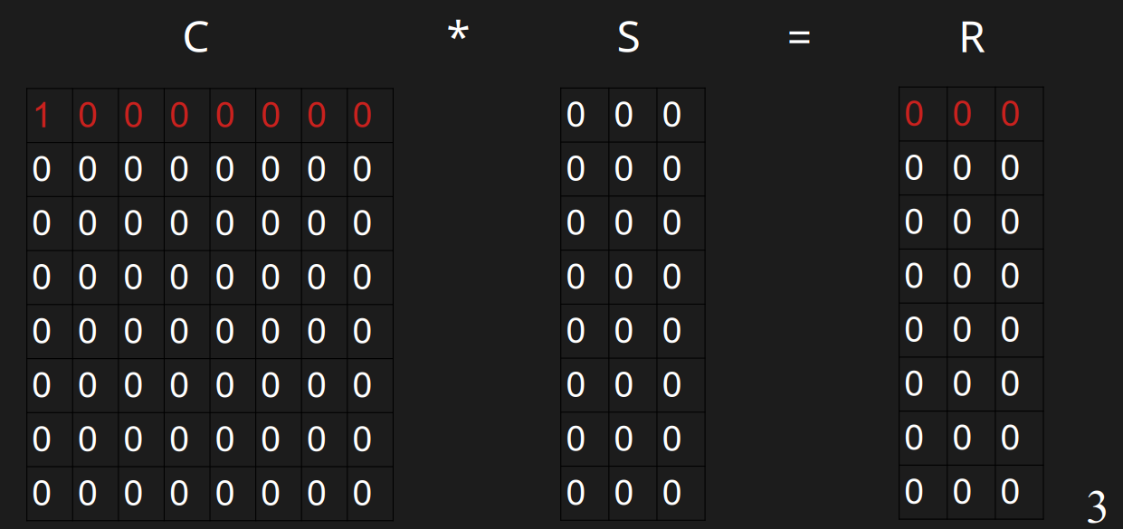插入u 插入u的时候，此时它开头的0的数量是0，需要插入到第0行。第0行都是0，直接插入即可。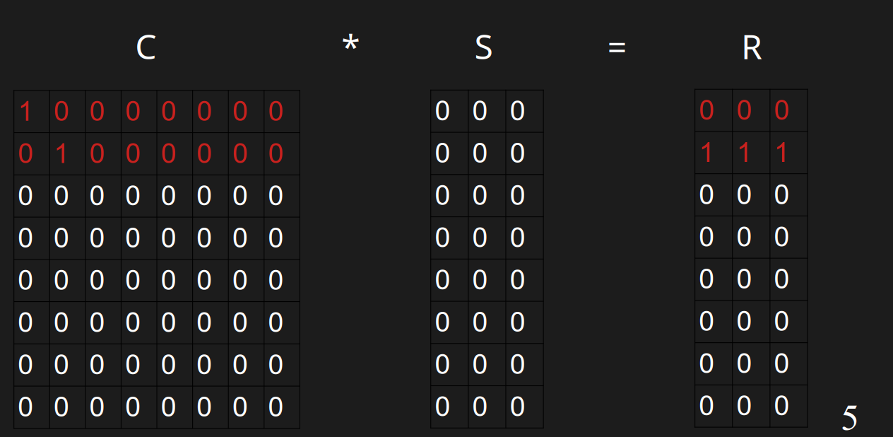  ### 插入v 插入v的时候，此时它开头的0的数量是1，需要插入到第0行。第0行已经有值了，h(v)=11000000与r(v)=111分别与第0行异或，得到01000000与111。此时它开头的0的数量是1，需要插入到第1行，可以直接插入。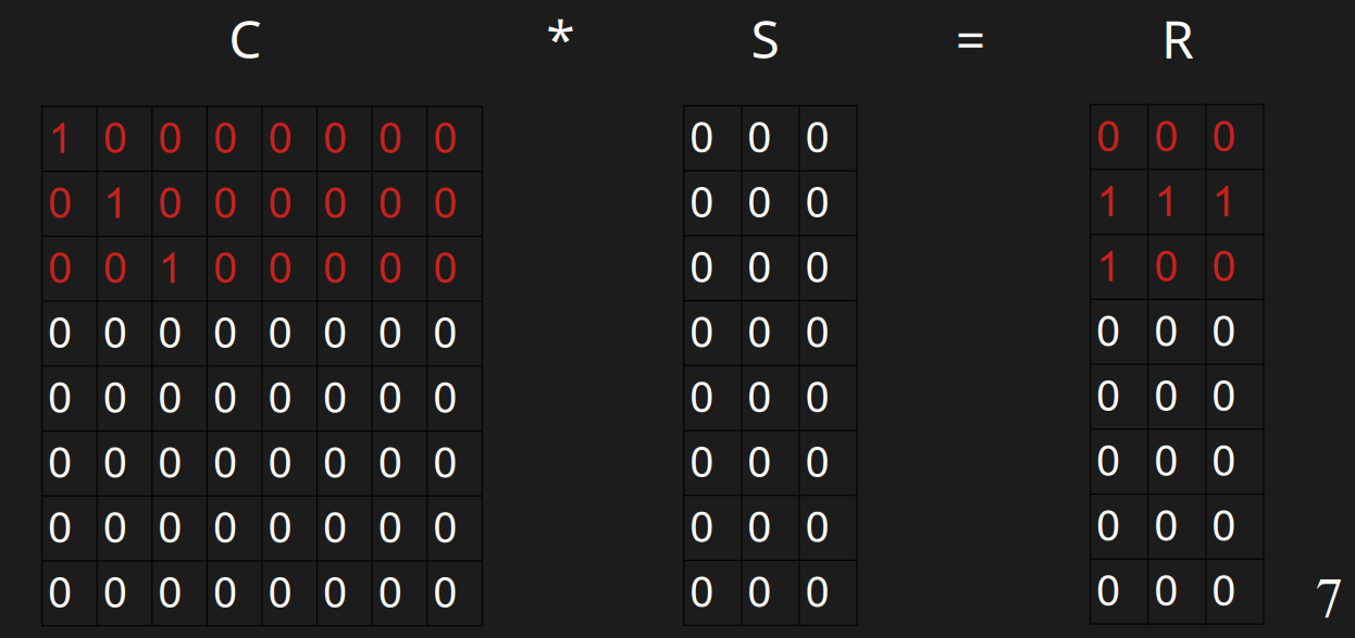  #### 插入w 插入w的时候，h(w)=10100000,r(w)=100，此时它开头的0的数量是0，需要插入到第0行。发现第0行有值了，分别与第0行异或，得到00100000与100，此时它开头的0的数量是2，此时需要插入到第2行。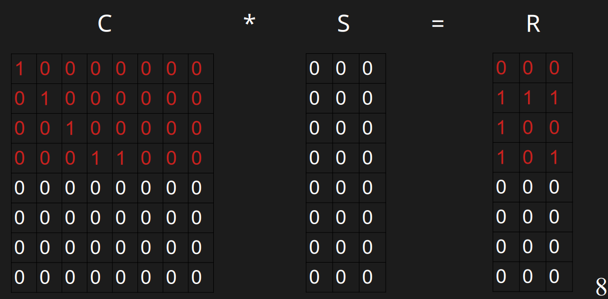  #### 插入x 插入x的时候，h(x)=00011000,r(x)=100，此时它开头的0的数量是3，需要插入到第3行，插入到第3行。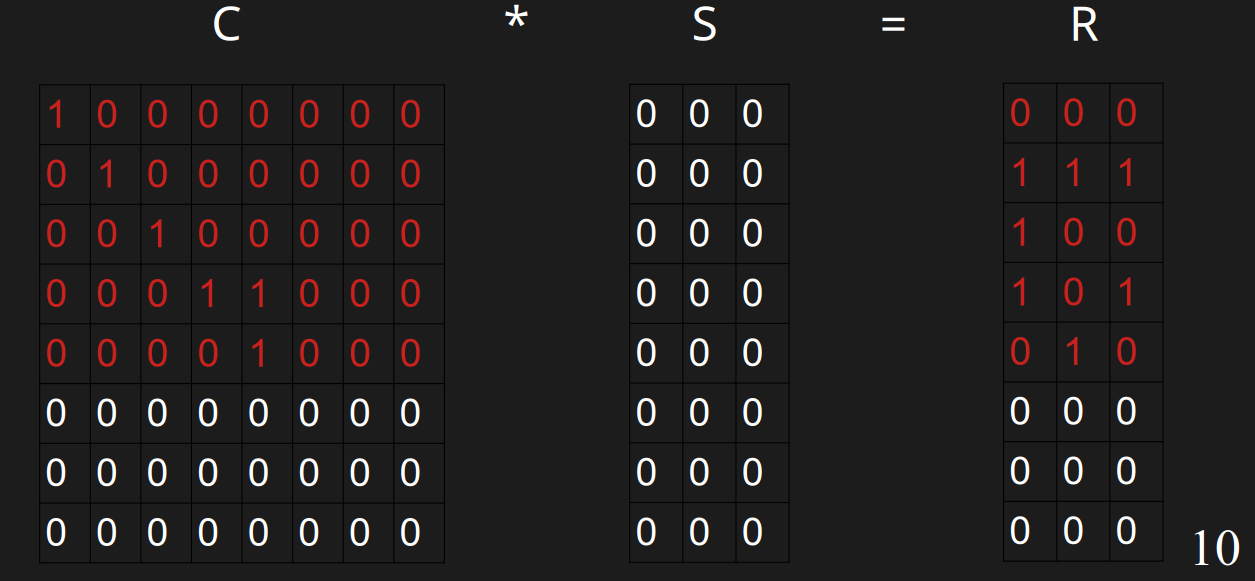  #### 插入y 插入y的时候，h(w)=10010000,r(w)=111，此时它开头的0的数量是0，需要插入到第0行。 发现第0行有值了，分别与第0行异或，得到00010000与111，此时它开头的0的数量是3，此时需要插入到第3行。 发现第3行有值了，分别与第3行异或，得到00001000与010，此时它开头的0的数量是4，此时需要插入到第4行。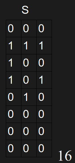  ### 解矩阵S 现在有C和R了，可以用线性代数的方法解S的值。但是由于C是上三角矩阵，且中间长度w=4的01串以外的地方都是0，所以我们可以从下往上计算，且只需要看其中4个值。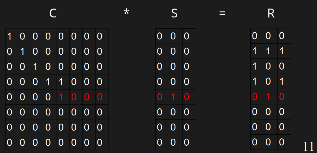 #### 解S的第4行 解这一行本质上是计算\(00001000\*S=010\)，即： \[0 \and S\_{0,0} \oplus 0 \and S\_{1,0} \oplus 0 \and S\_{2,0} \oplus 0 \and S\_{3,0} \oplus 1 \and S\_{4,0} \oplus 0 \and S\_{5,0} \oplus 0 \and S\_{6,0} \oplus 0 \and S\_{7,0} = 0 \] \[0 \and S\_{0,1} \oplus 0 \and S\_{1,1} \oplus 0 \and S\_{2,1} \oplus 0 \and S\_{3,1} \oplus 1 \and S\_{4,1} \oplus 0 \and S\_{5,1} \oplus 0 \and S\_{6,1} \oplus 0 \and S\_{7,1} = 1 \] \[0 \and S\_{0,2} \oplus 0 \and S\_{1,2} \oplus 0 \and S\_{2,2} \oplus 0 \and S\_{3,2} \oplus 1 \and S\_{4,2} \oplus 0 \and S\_{5,2} \oplus 0 \and S\_{6,2} \oplus 0 \and S\_{7,2} = 0 \] 由于C是上三角矩阵，且其中只有连续的4个wit可能为1，其他都为0，所以上面的计算可以化简为： \[1 \and S\_{4,0} \oplus 0 \and S\_{5,0} \oplus 0 \and S\_{6,0} \oplus 0 \and S\_{7,0} = 0 \] \[1 \and S\_{4,1} \oplus 0 \and S\_{5,1} \oplus 0 \and S\_{6,1} \oplus 0 \and S\_{7,1} = 1 \] \[1 \and S\_{4,2} \oplus 0 \and S\_{5,2} \oplus 0 \and S\_{6,2} \oplus 0 \and S\_{7,2} = 0 \] 由于C的最后三行是0，所以进一步化简为： \[1 \and S\_{4,0} = 0 \] \[1 \and S\_{4,1} = 1 \] \[1 \and S\_{4,2} = 0 \] 很容易解出来S的第四行  #### 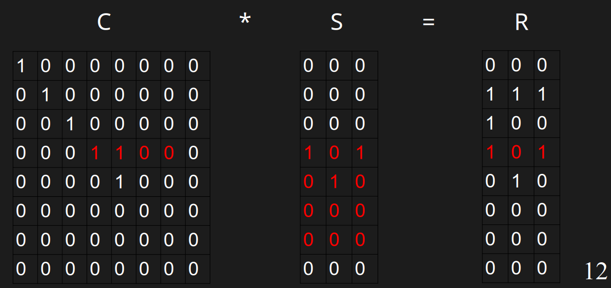解S的第3行 计算 \[0 \and S\_{0,0} \oplus 0 \and S\_{1,0} \oplus 0 \and S\_{2,0} \oplus 1 \and S\_{3,0} \oplus 1 \and S\_{4,0} \oplus 0 \and S\_{5,0} \oplus 0 \and S\_{6,0} \oplus 0 \and S\_{7,0} = 1 \] \[0 \and S\_{0,1} \oplus 0 \and S\_{1,1} \oplus 0 \and S\_{2,1} \oplus 1 \and S\_{3,1} \oplus 1 \and S\_{4,1} \oplus 0 \and S\_{5,1} \oplus 0 \and S\_{6,1} \oplus 0 \and S\_{7,1} = 0 \] \[0 \and S\_{0,2} \oplus 0 \and S\_{1,2} \oplus 0 \and S\_{2,2} \oplus 1 \and S\_{3,2} \oplus 1 \and S\_{4,2} \oplus 0 \and S\_{5,2} \oplus 0 \and S\_{6,2} \oplus 0 \and S\_{7,2} = 1 \] 由于C是上三角矩阵，且其中只有连续的4个bit可能为1，其他都为0，所以上面的计算可以化简为： \[1 \and S\_{3,0} \oplus 1 \and S\_{4,0} \oplus 0 \and S\_{5,0} \oplus 0 \and S\_{6,0} = 1 \] \[1 \and S\_{3,1} \oplus 1 \and S\_{4,1} \oplus 0 \and S\_{5,1} \oplus 0 \and S\_{6,1} = 0 \] \[1 \and S\_{3,2} \oplus 1 \and S\_{4,2} \oplus 0 \and S\_{5,2} \oplus 0 \and S\_{6,2} = 1 \] 容易算出S的第3行是101  #### 以此类推，计算完S  ## 查询过程 查询过程即判断表达式\(h(x)S=r(x)\)。 查询\(h(a)=11000000\)与\(r(a)=110\)，\(h(a)S=111\)，与r(a)不同，判定为不存在，查询结果正确 查询\(h(y)=10010000\)与\(r(y)=111\)，\(h(y)S=101\)，与r(y)不同，出现假阴性 查询\(h(b)=01000000\)与\(r(b)=111\)，得到101，与r(b)不同，出现假阳性 查询\(h(u)=11000000\)与\(r(u)=111\)，得到111，与r(u)相同，判定为存在，结果正确 ## 优化 ### 矩阵存储优化 可以发现，ribbon过滤器完全可以用一个\(w\*n\)的矩阵表示整个C，并且构建完S后完全可以丢弃C和R，所以只会在构建过中存在临时的空间消耗。 ### 构建、查询耗时优化 可以发现h(x)只有中间连续w个bit是有用的，所以查询时可以遍历S中的w行即可。 ### 假阳性率定制 假阳性率是\(2^{-w}\)，至于如何定制，这是论文中的内容了，如图，我们将w个 bit 连续存放，每m个w bit 为一组。所以整体看是 column-major 的，而每一组实际上是 row-major 的。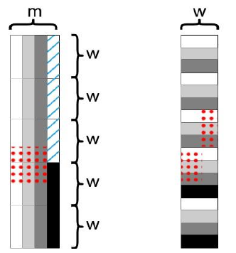这种混合方式称为 ICML(Interleaved Column-MajorLayout)  代码中，我们还需要特殊处理跨组（图中红点部分）的问题。对于 ICML 开始一段不足m列的特殊情况（图中蓝色斜线部分），我们可以忽略它。这样我们就可以存储 7、9、10bit 一行的矩阵。平均 3.4bit 一行的矩阵也是可行的，图中m = 4，但是前面三段都是使用m = 3，这样平均就是 3.4bit 一行了。 ### 提防假阴性 从前面查询的例子我们可以发现，过滤器存在假阴性，即实际插入位置不在$$[s(x),s(x)+w-1]$$范围内，这是要避免的。为了确保假阴性率极低，需要多分配一些内存。比如插入t个key，那么实际要分配的行数是需要多于t的。具体的假阴性率真不知道怎么算，在代码中是设置为一个值来规避的。这个值是 \[ 1-0.0251 + ln(t) \* 1.4427 \* 0.0083或1-0.0176 + ln(t) \* 1.4427 \* 0.0038; \] 算法导论有关于线性探测哈希表的讨论。如果w=64，那么期望探测到64次，load-factor需要是\(64=1/(1-a)\)，解出来loadfactor为63/64，即0.98，而这个公式在\(t=30,000,000\)时算出来是0.83左右